Understanding the outputs#
This page describes the outputs of the standard sampler and how to interpret them.
Logging output#
If the logger has been configured, the sampler will output various information
to the terminal and/or log file. By default, the logging level is set to
INFO which will output the progress of the sampler and any warnings or
errors.
By default, the sampler with log every nlive iterations and the log will
look something like this:
12-20 12:26 nessai INFO    : it:  6000: Rolling KS test: D=0.0325, p-value=0.0143
12-20 12:26 nessai INFO    : it:  6000: n eval: 23744 H: 3.10 dlogZ: 4.172 logZ: -8.996 +/- 0.039 logLmax: -1.84
The first line summarises the results of the Kolmogorov-Smirnov test for the insertion indices. The second line shows the following:
n evalis the total number of likelihood evaluationsHis the current informationdlogZis the change in log-evidence, this is used as the stopping criterionlogZis the current log-evidencelogLmaxis the maximum log-likelihood
Configuring logging#
The logger is configured via the nessai.utils.logging.configure_logger() function.
This allows the user to change logging level, output file and format as well as
some other options. For more information see documentation for the function.
The logging output from the sampler can also be configured to change its verbosity and frequency. This is done via the following options:
log_on_iterationsets whether the sampler logs on iteration or time.logging_intervalsets the interval at which the sampler logs information. Iflog_on_iterationis set toTrue, the sampler will log everylogging_intervaliterations. Iflog_on_iterationis set toFalse, the sampler will log everylogging_intervalseconds.
These options can be passed when configuring the sampler. The standard sampler and importance nested sampler have different defaults for these options.
Output files#
The sampler will output various files to the output directory. These include files describing the sampler configuration, a result file, files for resuming the sampler and various plots (see Plots). The specific files are:
config.json- A JSON file containing the configuration of the sampler.result.hdf5or result.json - A file containing the results of the sampler. The default format is hdf5 but this can be changed to json by setting result_extension=’json’ in the sampler configuration.nested_sampler_resume.pkl- A pickle file containing the state of the sampler which can be used to resume the sampler.
There are also various subdirectories which are created by the sampler:
proposal- Contains the proposal config (flow_config.json), file for resuming (model.pt) and any plots that are enabled.diagnostics- Contains additional diagnostic plots.
Plots#
If plot=True, the sampler will automatically generate various plots
which are saved in the output directory. These plots are useful for checking
the convergence of the sampler and the quality of the samples.
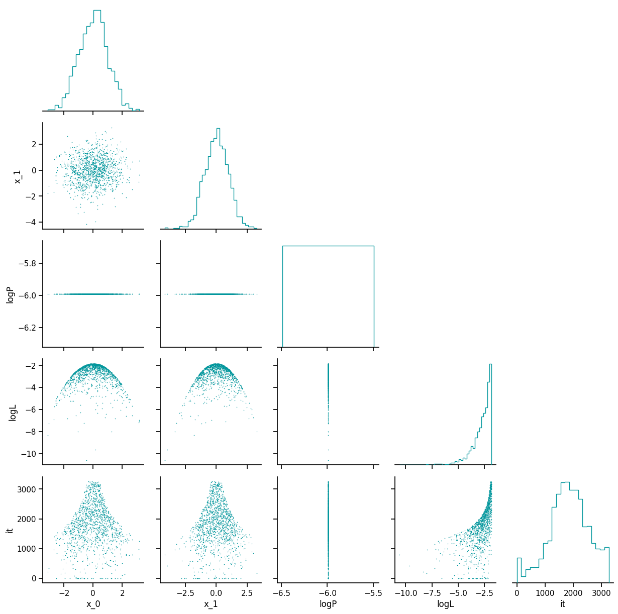
Posterior distribution#
The posterior distribution is plotted in posterior_distribution.png, this
includes the distributions for the parameters that were sampled and the
distribution of the log-prior, log-likelihood and the iteration at which the
sample was drawn.
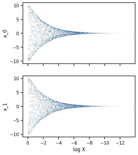
Trace#
The trace plot shows the nested samples for each parameter as a function of the log-prior volume. Whilst the sampler is running, the current live points will be shown in red.
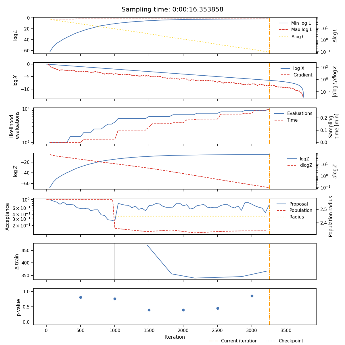
State#
The state plot shows all the statistics which are tracked during sampling as a function of iteration. From top to bottom these are
The minimum and maximum log-likelihood of the current set of live points
The cumulative number of likelihood evaluations
The current log-evidence \(\log Z\) and fraction change in evidence \(\text{d}Z\)
The acceptance of the population and proposal stages alongside the radius use for each population stage.
The \(p\)-value of the insertion indices every
nlivelive points
The iterations at which the normalising flow has been trained are indicated with vertical lines and total sampling-time is shown at the top of the plot.
Insertion indices#
The distribution of the insertion indices for all of the nested samples is shown on the left along with the expect uniform distribution and the 1-sigma bounds determined by the total number of live points.
The middle and right-hand plots show the difference between the analytic and estimated cumulative mass functions. The middle plot shows the difference between the CMFs for the entire run and the right-hand plot shows the difference for 8 equally sized sections of the run, lighter colours indicate later sections.
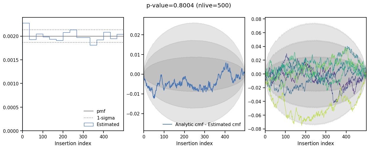
This plot is useful when checking if the sampler is correctly converged, a non-uniform distribution indicates the sampler is either under or over-constrained.
Diagnostic plots#
Additional diagnostic plots are saved in the diagnostics directory. These show
the distribution of the insertion indices every nlive iterations.